


MATRIX ALGEBRA:DETERMINANTS,INVERSES,EIGENVALUES
§C.2 SINGULAR MATRICES, RANK
If the determinant |A| of a n × n square matrix A ≡ An
is zero, then the matrix is said to be singular.
This means that at least one row and one column are linearly dependent on the
others. If this row
and column are removed, we are left with another matrix, say An-1, to
which we can apply the same
criterion. If the determinant |An-1| is zero, we can remove another
row and column from it to get An-2,
and so on. Suppose that we eventually arrive at an r × r matrix Ar
whose determinant is nonzero.
Then matrix A is said to have rank r , and we write rank(A) = r .
If the determinant of A is nonzero, then A is said to be nonsingular. The rank
of a nonsingular n × n
matrix is equal to n.
Obviously the rank of AT is the same as that of A since it is only
necessary to transpose “row” and
”column” in the definition.
The notion of rank can be extended to rectangular matrices as outlined in
section §C.2.4 below. That
extension, however, is not important for the material covered here.
EXAMPLE C.5
The 3 × 3 matrix
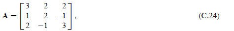
has rank r = 3 because |A| = −3 ≠ 0.
EXAMPLE C.6
The matrix
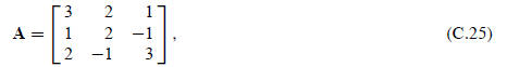
already used as an example in §C.1.1 is singular because
its first row and column may be expressed as linear
combinations of the others through the relations (C.9) and (C.10). Removing the
first row and column we are left
with a 2 × 2 matrix whose determinant is 2 × 3 − (−1) × (−1) = 5 ≠ 0.
Consequently (C.25) has rank r = 2.
§C.2.1 Rank Deficiency
If the square matrix A is supposed to be of rank r but in
fact has a smaller rank
 < r , the matrix is
said to be rank deficient. The number r −
 > 0 is called the rank deficiency.
EXAMPLE C.7
Suppose that the unconstrained master stiffness matrix K of a finite element has
order n, and that the element
possesses b independent rigid body modes. Then the expected rank of K is r = n −
b. If the actual rank is less
than r , the finite element model is said to be rank-deficient. This is an
undesirable property.
EXAMPLE C.8
An an illustration of the foregoing rule, consider the two-node, 4-DOF plane
beam element stiffness derived in
Chapter 13:
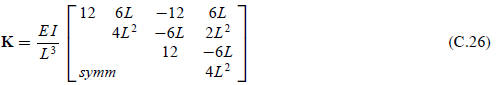
where E I and L are nonzero scalars. It can be verified
that this 4 × 4 matrix has rank 2. The number of rigid
body modes is 2, and the expected rank is r = 4 − 2 = 2. Consequently this model
is rank sufficient.
§C.2.2 Rank of Matrix Sums and Products
In finite element analysis matrices are often built
through sum and product combinations of simpler
matrices. Two important rules apply to “rank propagation” through those
combinations.
The rank of the product of two square matrices A and B cannot exceed the
smallest rank of the
multiplicand matrices. That is, if the rank of A is ra and the rank
of B is rb,
Rank(AB) ≤ min (C.27)
Regarding sums: the rank of a matrix sum cannot exceed the
sum of ranks of the summand matrices.
That is, if the rank of A is ra and the rank of B is rb,

§C.2.3 Singular Systems: Particular and Homegeneous Solutions
Having introduced the notion of rank we can now discuss
what happens to the linear system (C.16)
when the determinant of A vanishes, meaning that its rank is less than n. If so,
the linear system (C.16)
has either no solution or an infinite number of solution. Cramer’s rule is of
limited or no help in this
situation.
To discuss this case further we note that if |A| = 0 and
the rank of A is r = n − d, where d ≥ 1 is the
rank deficiency, then there exist d nonzero independent vectors zi ,
i = 1, . . . d such that
Azi = 0. (C.29)
These d vectors, suitably orthonormalized, are called null
eigenvectors of A, and form a basis for its
null space.
Let Z denote the n × d matrix obtained by collecting the zi
as columns. If y in (C.13) is in the range
of A, that is, there exists an nonzero xp such that y = Axp,
its general solution is

where w is an arbitrary d × 1 weighting vector. This
statement can be easily verified by substituting
this solution into Ax = y and noting that AZ vanishes.
The components xp and xh are called
the particular and homogeneous part, respectively, of the solution
x. If y = 0 only the homogeneous part remains.
If y is not in the range of A, system (C.13) does not
generally have a solution in the conventional
sense, although least-square solutions can usually be constructed. The reader is
referred to the many
textbooks in linear algebra for further details.
§C.2.4 Rank of Rectangular Matrices
The notion of rank can be extended to rectangular
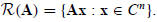
matrices, real or complex, as follows. Let A be m×n. Its column
range space
 is the subspace spanned by Ax where x is the set of all complex n-vectors.
Mathematically:
is the subspace spanned by Ax where x is the set of all complex n-vectors.
Mathematically:
 The rank r of A is the dimension of

The null space
 of A is the set of n-vectors z such that Az = 0. The dimension of
 is n − r .
Using these definitions, the product and sum rules (C.27)
and (C.28) generalize to the case of rectangular (but
conforming) A and B. So does the treatment of linear equation systems Ax = y in
which A is rectangular; such
systems often arise in the fitting of observation and measurement data.
In finite element methods, rectangular matrices appear in
change of basis through congruential transformations,
and in the treatment of multifreedom constraints.