


Solving Systems of Linear Equations
The following pages contain some instructions on the usage of the TI-83/83
Plus
graphing calculator.
The example used below is taken out of the text titled “College Algebra -
Enhanced with
Graphing Utilities, 3rd Edition” by Sullivan and Sullivan, III.
Example#3 Solving a System of Linear Equations p. 515: Solve the
following system of
equations.
2x + y = 5 (1)
− 4x + 6y =12 (2)
First, each equation in the above system must be solved for y (i.e., written
in slope-intercept
form) before it can be entered into function Editor
 .
Hence, the system of
.
Hence, the system of
equations to be entered into the graphing calculator becomes:
Press
to go into the function Editor menu. If you have any previously entered
functions showing up on the function editor menu, press
 to move the cursor down by
that function, and press
 delete it.
While the blinking cursor is by \Y1 =, start entering the expression − 2x + 5
, which is the
right side of the first equation. Press  . Type in 2. Press
 for the generic input
variable x. Press  . Type in 5. At this point, your screen should look like the
screen on
. Type in 5. At this point, your screen should look like the
screen on
the left given below.
Press  to move the
cursor down by \Y2 =. Start entering the expression
to move the
cursor down by \Y2 =. Start entering the expression
 which
which
is the right side of the second equation. Press
 Type in 2. Press
 Type in 3. Press
 . Press
  for the generic input variable x. Press
  .
Type in 2. At this point,
.
Type in 2. At this point,
your screen should look like the screen on the right given above.
The solution of this system of linear equations is the
same as the points of intersection of
the graphs of the equations, which have been entered into the \Y1 = and \Y2
= locations of
the function editor, respectively. Press
 to type in the following WINDOW
settings, which are given on the left below. Press
 see the two graphs. At this
point, your screen should look like the screen on the right given below.
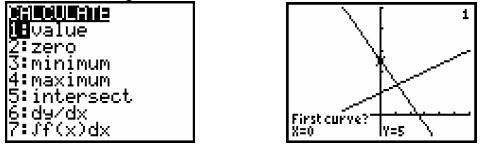
From the graph on the right above, there appears to be a
point of intersection of these two
graphs, which means the system is consistent and the equations are independent.
Press  and
and  to access the CALC menu. At this point, your screen should
look like the screen on the left given below.
Press  four times to
move the cursor down to 5:intersect and press
four times to
move the cursor down to 5:intersect and press
 to select
this option from the CALCULATE menu. At this point, your screen should look like
the
screen on the right given above with the calculator prompting you for the First
Curve?.
Be sure that the blinking trace cursor is on the first graph, which is indicated
by a small 1
showing up in the upper-right corner. Press  to confirm. At this point, your screen
should look like the screen on the left given below with the calculator
prompting you for
the Second Curve?.
Be sure that the blinking trace cursor is on the second
graph, which is indicated by a
small 2 showing up in the upper-right corner. Press
 to confirm. At this point,
your screen should look like the screen on the right given above with the
calculator
prompting you for a Guess? value for the point of intersection of the two
graphs. Type in
1 for a guess value of the point of intersection. At this point, your screen
should look like
the screen on the left given below. Press  to
see that the location of the
to
see that the location of the
intersection point of these two graphs. At this point, your screen should look
like the
screen on the right given below.
The intersection point of these two graphs or the solution
of this linear system of
equations is obtained as (1.125, 2.75).